Export anomaly model

Once the anomaly segmentation session run is complete, you can export the docker model and download it locally or on a different machine.

Export Model

In the model screen, click the Export Model button. If you want to apply a custom rule in the exported model, then load that rule by clicking the Saved Rules button.

Once the model gets exported, the button label is displayed as Download Model.
Click the Download Model button.

You can click the Download Model button to download the docker image. Follow the necessary steps as mentioned in the next section to extract the docker image and run the docker.

Download Model

Click Download Model to view the available download options as shown below.
1. Copy URL: Click the copy icon to copy the URL of the exported model to download it on a different machine.
2. Copy Path: Click the copy icon to copy the image path and follow the instruction by using the required credentials.
3. Download: Click this option to download the exported model to the same system.

X86-64 support
The downloaded docker image can run only on X86-64 hardware and specifically does not support the ARM based Mac M1 and similar architectures.

The next sections explain how to use the downloaded docker for inference.

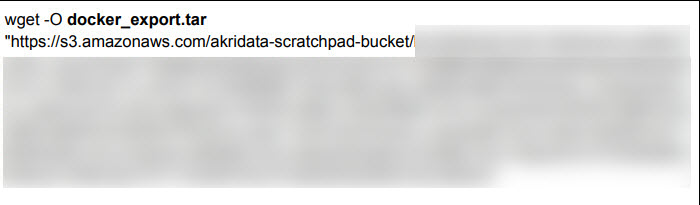
Download Docker image using Copy URL

Click the copy icon to copy the URL of the export model and download it on a different machine.
Load the exported model as docker image, using the following command:
```
docker load -i <exported.tar file>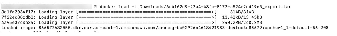
```
The command prompt displays the docker image name under REPOSITORY.
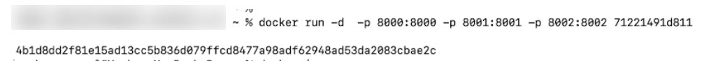
Run the docker container, using the following command:
Verify if the container is running, using the following command:
```
docker ps command.
```

Run Inference

The downloaded docker image adheres to kserve inference server interface. The following steps describe running inference through kserve HTTP interface. The name of the kserve model is ‘anoseg_ensemble’.

Check if the model is available by using the following command:
```
curl http://localhost:8000/v2/models/anoseg_ensemble
```
This should display the metadata for the model, as follows.
Create input.json for the inference.
1. id: Any string to identify this specific inference.
2. parameters
  1. frame_height and frame_width: Image height and width in pixels.
  2. frame_type: Input image file format (e.g., jpeg, png)
3. inputs
  1. name: Must be “INPUT_IMG”
  2. shape: 1-D array with size of the image file. In the below example, the image file size is 35581 bytes.
  3. datatype: Must be UINT8
  4. data: The bytes array filled by reading the image file.
```
{
  "id": "inference_request_001",
  "parameters": {
    "frame_height": 512,
    "frame_width": 512,
    "frame_type": "jpeg"
  },
  "inputs": [
    {
      "name": "INPUT_IMG",
      "shape": [35581],
      "datatype": "UINT8",
      "parameters": {},
      "data": [255, 216, 255, 224, 0, 16, 74, 70, 73, 70, 0, 1, 1, 1, 0, 96, 0, 96, 0, 0, ...]
    }
  ]
}
```

Run inference by invoking the REST endpoint. A curl command example is provided below.

curl -X POST http://localhost:8000/v2/models/anoseg_ensemble/infer \
     -H "Content-Type: application/json" \
     -d @${HOME}/Downloads/input.json > result.json

The kserve inference displays the following output as a response:

"outputs": [
  {
    "name": "OUTPUT_LABELS",
    "datatype": "FP32",
    "shape": [-1]
  },
  {
    "name": "OUTPUT_SCORES",
    "datatype": "FP32",
    "shape": [-1]
  },
  {
    "name": "OUTPUT_AMAP_IMAGE",
    "datatype": "UINT8",
    "shape": [-1]
  }
]

“shape”: [-1] indicates variable-length output, depending on the image size or compression.

The output field descriptions are as follows:

Output Name	Data Type	Description
OUTPUT_LABELS	FP32	Predicted label. 0 = Normal, 1 = Anomaly
OUTPUT_SCORES	FP32	Confidence score for the predicted label. Range 0.0 to 1.0
OUTPUT_AMAP_IMAGE	UINT8	Flattened JPEG image (as byte array) showing the visual anomaly heatmap.

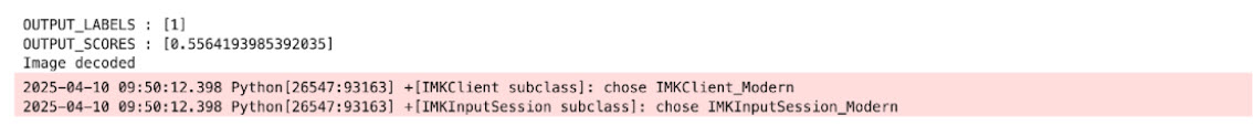
An example inference response would be as follows:

{
  "model_name": "anoseg_ensemble",
  "outputs": [
    {
      "name": "OUTPUT_LABELS",
      "datatype": "FP32",
      "shape": [1],
      "data": [1.0]
    },
    {
      "name": "OUTPUT_SCORES",
      "datatype": "FP32",
      "shape": [1],
      "data": [0.9123]
    },
    {
      "name": "OUTPUT_AMAP_IMAGE",
      "datatype": "UINT8",
      "shape": [13248],
      "data": [255, 216, 255, 224, ...]  // JPEG byte array
    }
  ]
}

A sample program to visualize the anomaly maps for labels, score and heatmap, is shown below.

import json
import numpy as np
import cv2

with open("result.json", "r") as f: # FIle path for result.json 
    result = json.load(f)

output = result["outputs"]
amap_output = next(x for x in output if x["name"] == "OUTPUT_AMAP_IMAGE")
amap_bytes = np.array(amap_output["data"], dtype=np.uint8)
OUTPUT_SCORES = next(x for x in output if x["name"] == "OUTPUT_SCORES")["data"]

OUTPUT_LABELS = next(x for x in output if x["name"] == "OUTPUT_LABELS")["data"]

decoded_img = cv2.imdecode(amap_bytes, cv2.IMREAD_COLOR)
print(f"OUTPUT_LABELS : {OUTPUT_LABELS}")
print(f"OUTPUT_SCORES : {OUTPUT_SCORES}")

if decoded_img is None:
    print("Failed to decode image")
else:
    print("Image decoded")
    cv2.imshow("Anomaly Heatmap", decoded_img)
    cv2.waitKey(0)
    cv2.destroyAllWindows()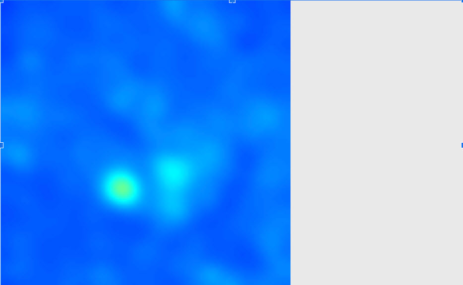

The labels and scores will appear as follows: